What is string art?

String art is a technique that involves weaving threads between fixed points/nails to form patterns by playing with the manner in which threads intersect each other. These fixed-points/nails are typically arranged along the edge of a circular frame and by connecting specific nails with threads that travel along straight lines, the overlap can be tuned, gradually building up a recognizable image or a pattern. This art form was invented in the late 19th century by Mary Everest Boole, an English mathematician. She came up with this technique as an educational tool to help children understand mathematical concepts such as geometry through hands-on learning.

What makes string art particularly interesting is its use of simple geometric shapes and linear structures to approximate complex forms. Each thread is just a straight line, but by layering many lines at different angles, intricate shapes and gradients can emerge. This process can be thought of as the construction of an image through a series of basic building blocks. In this blog post, we will delve into the mathematical ideas behind string art. We will examine how geometry and linear algebra play a crucial role in determining the best arrangement of threads to approximate a given image. Additionally, we will provide a step-by-step explanation of an algorithm that automates the process, making it easier to design and recreate string art using computational tools.

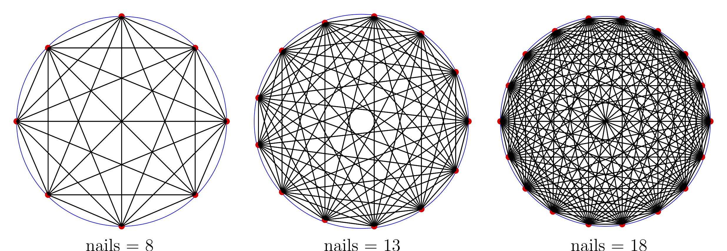String art configurations with 8, 13, and 18 nails. Here each nail along the circle is connected to every other nail. We see that by increasing the number of nails leads to complex geometric patterns, demonstrating the ability of string art to approximate intricate shapes through simple linear elements.

Mathematical foundation

Representation of threads as basis functions

Each thread is defined as a line segment connecting two points on the circle. Mathematically, the equation of a line between two points $(x_0, y_0)$ and $(x_1, y_1)$ is given by: $\vec{r}(t) = (1 - t) \begin{bmatrix} x_0 \\ y_0 \end{bmatrix} + t \begin{bmatrix} x_1 \\ y_1 \end{bmatrix}, \quad t \in [0, 1].$

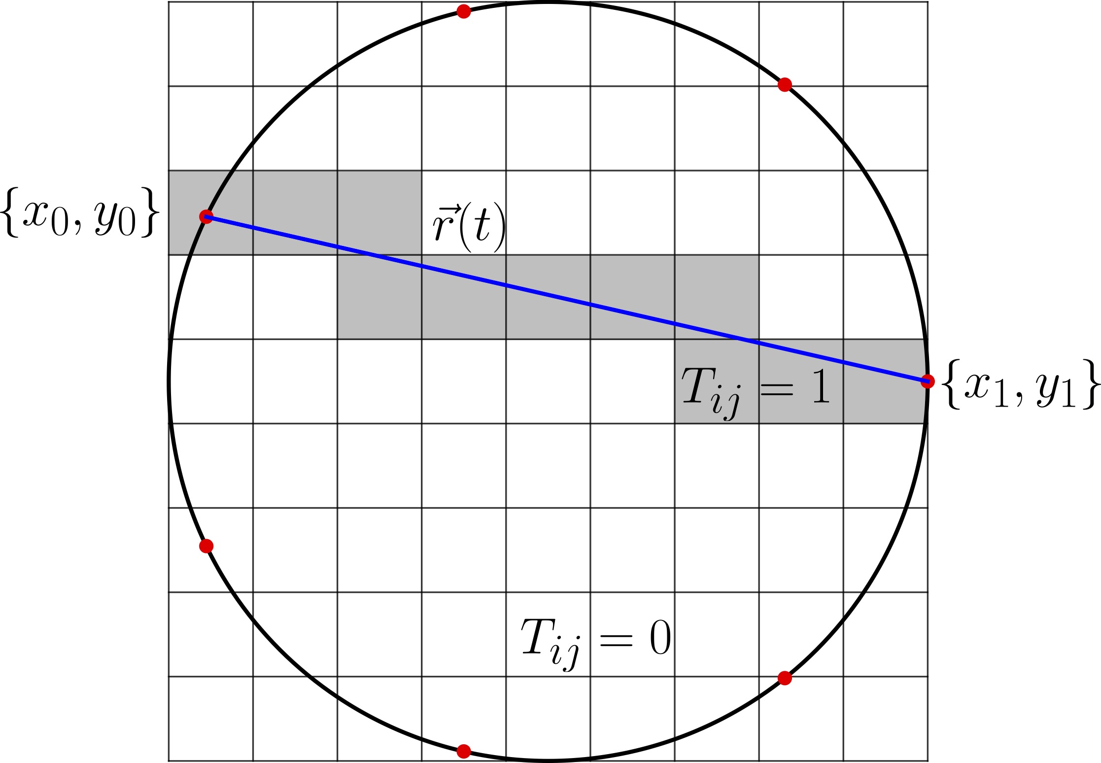
A visual representation of the thread intensity matrix $T$ for a single thread (denoted by blue line) connected between two nails(denoted by red dots). The pixels which have an intersection with the thread are assigned value $T_{ij}=1$, while the other pixels of the grid are assigned values $T_{ij}=0$.

Thread intensity matrix

Each thread can be represented as a binary vector, where each entry corresponds to a pixel on the grid. If the pixel lies on the thread, the entry is 1; otherwise, it is 0. Collecting all such thread vectors forms the thread intensity matrix, $T \in \mathbb{R}^{n \times m}$ with $n$ being the total number of pixels in the image grid, $m$ is the total number of threads, determined by the number of connected nails. If there are $k$ nails with all of them connected, then $m = k(k-1)$, as each pair of nails represents a unique thread. Each column of $T$ corresponds to a thread, and each row corresponds to a pixel in the grid. The value $T_{ij}$ is 1 if thread $j$ passes through pixel $i$, and 0 otherwise.

Constructing $T$

For each thread connecting nails at $(x_0, y_0)$ and $(x_1, y_1)$,

• Iterate over all pixels $(p_x, p_y)$ in the image grid given by their pixel index.

• Compute the perpendicular distance of $(p_x, p_y)$ from the thread. To determine whether a pixel $(p_x, p_y)$ lies on this line, we calculate its perpendicular distance from the line, $d = \dfrac{|(p_x - x_0)(y_1 - y_0) - (p_y - y_0)(x_1 - x_0)|}{\sqrt{(y_1 - y_0)^2 + (x_1 - x_0)^2}}.$ If $d \leq \text{threshold}$, the pixel is considered part of the thread.

• If the distance satisfies the threshold condition, set the corresponding entry as $T_{ij} = 1$ if pixel $i$ is on thread $j$, otherwise $T_{ij} = 0$.

For a small grid and few threads, the thread intensity matrix may look like this: $T = \begin{bmatrix} 1 & 0 & 0 & \cdots \\ 1 & 1 & 0 & \cdots \\ 0 & 1 & 1 & \cdots \\ \vdots & \vdots & \vdots & \ddots \end{bmatrix}.$ Here each row corresponds to a pixel and each column corresponds to a thread. The ntries are 1 if the thread passes through the pixel. By constructing $T$, we create a mathematical representation of the threads' contributions to the image grid. This matrix serves as the basis for solving the linear system to reconstruct the target image.

Image reconstruction as a linear system

The reconstruction of an image in string art involves finding the optimal combination of threads that approximates the target image. Let us define the components and we will explain the reconstruction process in detail after the definitions.
Target image, $\vec{I}$: The target image is flattened into a vector $\vec{I}$ of size $n \times 1$, where each entry represents the grayscale intensity of a pixel. The goal is to approximate $\vec{I}$ using the contributions of the threads.
Thread weights, $\vec{w}$: The vector $\vec{w}$ of size $m \times 1$ contains the weights of the threads. Each weight $w_j$ determines the intensity or contribution of the thread $j$ to the reconstruction. These weights capture the importance of a specific feature in the image we would like to reconstruct and will become important soon.
Linear system representation: We can immediately see that by multiplying $T$ and $\vec{w}$, we get a flattened version of an image. The multiplication here simply telling us that the image $\vec{I}$ is constructed by a sum of threads from $T$ with weights $\vec{w}$. The reconstructed image is given by, $\vec{I}_{\text{reconstructed}} = T \vec{w},$ where $T$ is the thread intensity matrix of size $n \times m$, and $\vec{w}$, is the the weight vector of size $m \times 1$. The objective is to find $\vec{w}$ such that the reconstructed image $T \vec{w}$ closely matches the target image $\vec{I}$.

Minimizing reconstruction error:

Our goal is to construct a target image by a set of threads. The error between the constructed and target image is measured using the Euclidean norm give by, $\mathcal{E}(\vec{w}) = \|T \vec{w} - \vec{I}\|_2^2.$ The optimal weights $\vec{w}^*$ minimize this error for a given $T$, $\vec{w}^* = \arg \min_{\vec{w}} \|T \vec{w} - \vec{I}\|_2^2.$ This is a standard least squares problem, where the solution ensures the best possible approximation of $\vec{I}$ in terms of the thread contributions. By solving this optimization problem, we determine how much each thread contributes to the final reconstructed image.

Solving the optimization problem

The problem of minimizing the quadratic error, $\mathcal{E}(\vec{w}) = ||T \vec{w} - \vec{I}||_2^2$ can be solved mathematically using linear algebra. In our application, $T$ is the thread matrix composed of column vectors representing the contribution of each thread (or line) in the image, and $\vec{I}$ is the flattened target image.

Objective function

The quadratic/squared error can be written as, $\mathcal{E}(\vec{w}) = \|T \vec{w} - \vec{I}\|_2^2 = (T \vec{w} - \vec{I})^\top (T \vec{w} - \vec{I}).$ Expanding the product gives, $\mathcal{E}(\vec{w}) = \vec{w}^\top T^\top T \vec{w} - 2 \vec{I}^\top T \vec{w} + \vec{I}^\top \vec{I}.$ Since $\vec{I}^\top \vec{I}$ is a constant and does not depend on $\vec{w}$, it can be ignored during minimization.

Gradient of the objective function

To find the optimal weight vector $\vec{w}$ that minimizes $\mathcal{E}(\vec{w})$, we set the gradient with respect to $\vec{w}$ equal to zero, $\nabla_{\vec{w}} \mathcal{E}(\vec{w}) = 2T^\top T \vec{w} - 2T^\top \vec{I} = \vec{0}.$ Dividing by 2, we get the normal equation, $T^\top T \vec{w} = T^\top \vec{I}.$ If $T^\top T$ is invertible, the optimal weight vector $\vec{w}^*$ can be computed as, $\vec{w}^* = \left( T^\top T \right)^{-1} T^\top \vec{I}.$ In cases where $T^\top T$ is singular or ill-conditioned, the Moore-Penrose pseudoinverse provides a robust alternative, $\vec{w}^* = T^{+} \vec{I},$ with $T^{+}$ denoting the pseudoinverse of $T$.

Reconstruction

Once the weight vector $\vec{w}$ is obtained, the reconstructed image is formed as, $\vec{I}_{\text{reconstructed}} = T\vec{w}.$ Reshaping $\vec{I}_{\text{reconstructed}}$ back into the original grid produces the final string art representation.
This approach illustrates how linear algebra and numerical optimization methods can be harnessed to approximate complex images using simple geometric primitives.

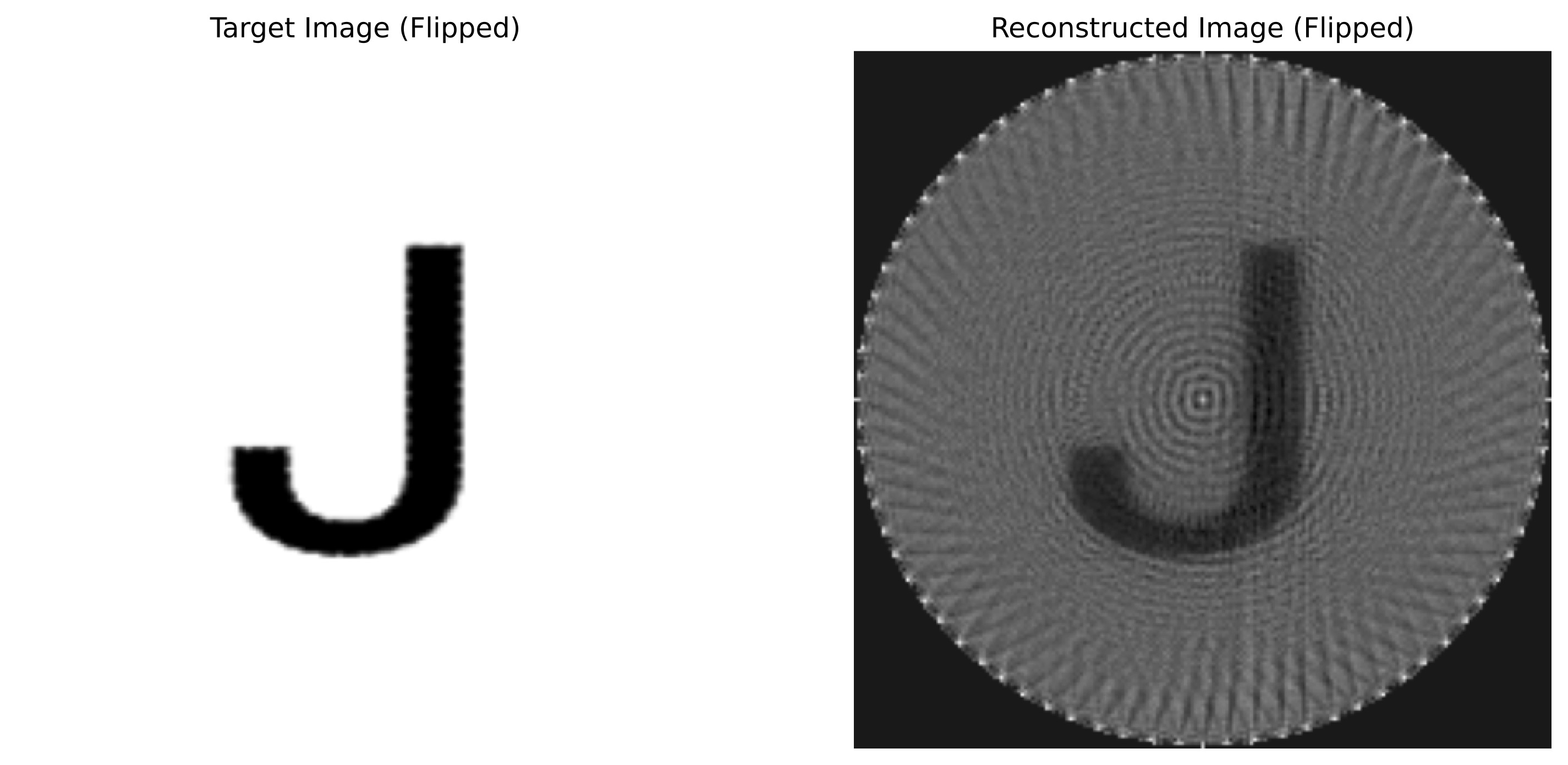
Reconstructed string art from an input PNG image using the technique described here. The left side shows the target image $\vec{I}$, while the right side demonstrates its reconstruction $\vec{I}_{\rm reconstructed}$ using weighted thread patterns.

Conclusion

String art beautifully combines art and mathematics. By understanding its geometric and algebraic principles, you can create stunning reconstructions of complex images. Do experiment with different configurations, numbers of nails, and target images to unleash your creativity with the python code attached here!